Batch Active Learning#
While it is possible to perform rudimentary data selection simply by randomly choosing samples, the batch of data thus drawn might not be the most informative one. Choosing those samples whith the largest prediction uncertainties from trajectories often results in the selection of configurations from subsequent time steps.
Batch selection methods can be constructed to select informative and diverse data, with or without following the underlying distribution.
We will illustrate this in a mock learning on the fly setup.
[1]:
from pathlib import Path
import yaml

from ase.md.velocitydistribution import MaxwellBoltzmannDistribution
from ase import units
from ase.md.langevin import Langevin
from ase.optimize.fire import FIRE
from ase.io.trajectory import TrajectoryWriter
from ase.io import read
import numpy as np
import matplotlib.pyplot as plt


from apax.bal import api
from apax.md import ASECalculator
from apax.utils.datasets import download_md22_benzene_CCSDT, mod_md_datasets
from apax.utils.helpers import mod_config
Dataset Acquisition#
[3]:
# Download CCSD(T) Data
data_path = Path("project")
cc_train_file_path, cc_val_file_path = download_md22_benzene_CCSDT(data_path)
cc_train_file_path = mod_md_datasets(cc_train_file_path)
cc_val_file_path = mod_md_datasets(cc_val_file_path)
Model Training#
Unlike simpler data selection methods, such as random selection, we first need to train a model. It is the representation learned by the model which will serve as the basis for our similarity metric.
[7]:
!apax template train
/home/ms/miniconda3/envs/apax311/lib/python3.11/pty.py:89: RuntimeWarning: os.fork() was called. os.fork() is incompatible with multithreaded code, and JAX is multithreaded, so this will likely lead to a deadlock.
  pid, fd = os.forkpty()
[10]:
config_path = Path("config.yaml")

config_updates = {
    "n_epochs": 200,
    "data": {
        "batch_size": 4,
        "valid_batch_size": 100,
        "experiment": "benzene",
        "directory": "project/models",
        "train_data_path": str(cc_train_file_path),
        "val_data_path": str(cc_val_file_path),
        "data_path": None,
        "energy_unit": "kcal/mol",
        "pos_unit": "Ang",
    },
}
config_dict = mod_config(config_path, config_updates)

with open("config.yaml", "w") as conf:
    yaml.dump(config_dict, conf, default_flow_style=False)
[11]:
!apax train config.yaml
/home/ms/miniconda3/envs/apax311/lib/python3.11/pty.py:89: RuntimeWarning: os.fork() was called. os.fork() is incompatible with multithreaded code, and JAX is multithreaded, so this will likely lead to a deadlock.
  pid, fd = os.forkpty()
INFO | 18:13:29 | Running on [cuda(id=0)]
INFO | 18:13:29 | Initializing Callbacks
INFO | 18:13:29 | Initializing Loss Function
INFO | 18:13:29 | Initializing Metrics
INFO | 18:13:29 | Running Input Pipeline
INFO | 18:13:29 | Read training data file project/benzene_ccsd_t-train_mod.xyz
INFO | 18:13:29 | Read validation data file project/benzene_ccsd_t-test_mod.xyz
INFO | 18:13:29 | Loading data from project/benzene_ccsd_t-train_mod.xyz
INFO | 18:13:29 | Loading data from project/benzene_ccsd_t-test_mod.xyz
INFO | 18:13:30 | Computing per element energy regression.
INFO | 18:13:30 | Initializing Model
INFO | 18:13:30 | initializing 1 models
INFO | 18:13:34 | Initializing Optimizer
INFO | 18:13:34 | Beginning Training
Epochs:   0%|                                                               | 0/200 [00:00<?, ?it/s]WARNING | 18:13:47 | SaveArgs.aggregate is deprecated, please use custom TypeHandler (https://orbax.readthedocs.io/en/latest/custom_handlers.html#typehandler) or contact Orbax team to migrate before May 1st, 2024. If your Pytree has empty ([], {}, None) values then use PyTreeCheckpointHandler(..., write_tree_metadata=True, ...) or use StandardCheckpointHandler to avoid TypeHandler Registry error. Please note that PyTreeCheckpointHandler.write_tree_metadata default value is already set to True.
Epochs: 100%|██████████████████████████████████| 200/200 [01:31<00:00,  2.18it/s, val_loss=0.000692]
INFO | 18:15:06 | Finished training
Molecular Dynamics / Data Generation#
Now we will create a pool of data to select new samples from. In order to emphasize the selection method used in the next section, we will combine MD and geometry optimization, a common occurrence in learning on the fly.
[40]:
atoms = read(str(cc_train_file_path), "0")
calc = ASECalculator("project/models/benzene")
atoms.calc = calc
[42]:
def printenergy(a=atoms):  # store a reference to atoms in the definition.
    """Function to print the potential, kinetic and total energy."""
    epot = a.get_potential_energy() / len(a)
    ekin = a.get_kinetic_energy() / len(a)
    print('Energy per atom: Epot = %.3feV  Ekin = %.3feV (T=%3.0fK)  '
          'Etot = %.3feV' % (epot, ekin, ekin / (1.5 * units.kB), epot + ekin))

writer = TrajectoryWriter("project/benzene.traj", "w", atoms)

MaxwellBoltzmannDistribution(atoms, temperature_K=298)
dyn = Langevin(atoms, 0.5*units.fs, temperature_K=298, friction=0.002)
dyn.attach(writer, interval=100)
dyn.attach(printenergy, interval=1000)
dyn.run(10000)

opt = FIRE(atoms)
opt.attach(writer)
opt.run()
Energy per atom: Epot = -524.783eV  Ekin = 0.042eV (T=322K)  Etot = -524.741eV
Energy per atom: Epot = -524.784eV  Ekin = 0.032eV (T=246K)  Etot = -524.752eV
Energy per atom: Epot = -524.786eV  Ekin = 0.037eV (T=287K)  Etot = -524.749eV
Energy per atom: Epot = -524.784eV  Ekin = 0.033eV (T=252K)  Etot = -524.752eV
Energy per atom: Epot = -524.786eV  Ekin = 0.040eV (T=307K)  Etot = -524.746eV
Energy per atom: Epot = -524.781eV  Ekin = 0.036eV (T=275K)  Etot = -524.746eV
Energy per atom: Epot = -524.783eV  Ekin = 0.038eV (T=295K)  Etot = -524.745eV
Energy per atom: Epot = -524.777eV  Ekin = 0.031eV (T=242K)  Etot = -524.745eV
Energy per atom: Epot = -524.772eV  Ekin = 0.038eV (T=292K)  Etot = -524.735eV
Energy per atom: Epot = -524.776eV  Ekin = 0.039eV (T=305K)  Etot = -524.736eV
Energy per atom: Epot = -524.788eV  Ekin = 0.055eV (T=427K)  Etot = -524.733eV
      Step     Time          Energy         fmax
FIRE:    0 18:31:17    -6297.460205        2.9797
FIRE:    1 18:31:17    -6297.640137        0.9522
FIRE:    2 18:31:17    -6297.634888        2.8176
FIRE:    3 18:31:17    -6297.690125        2.0002
FIRE:    4 18:31:17    -6297.744812        0.7309
FIRE:    5 18:31:17    -6297.752930        1.0354
FIRE:    6 18:31:17    -6297.754883        0.9791
FIRE:    7 18:31:17    -6297.759338        0.8737
FIRE:    8 18:31:17    -6297.764954        0.7249
FIRE:    9 18:31:17    -6297.770813        0.5532
FIRE:   10 18:31:17    -6297.776001        0.4649
FIRE:   11 18:31:17    -6297.780212        0.4568
FIRE:   12 18:31:17    -6297.783813        0.4434
FIRE:   13 18:31:17    -6297.788879        0.5014
FIRE:   14 18:31:17    -6297.794434        0.5313
FIRE:   15 18:31:17    -6297.801697        0.4645
FIRE:   16 18:31:17    -6297.810730        0.3380
FIRE:   17 18:31:17    -6297.818176        0.2703
FIRE:   18 18:31:17    -6297.823425        0.2700
FIRE:   19 18:31:17    -6297.829163        0.3942
FIRE:   20 18:31:17    -6297.834229        0.3305
FIRE:   21 18:31:17    -6297.838928        0.2279
FIRE:   22 18:31:17    -6297.841248        0.3689
FIRE:   23 18:31:17    -6297.845642        0.3514
FIRE:   24 18:31:17    -6297.849121        0.2314
FIRE:   25 18:31:17    -6297.850342        0.3102
FIRE:   26 18:31:17    -6297.850586        0.2551
FIRE:   27 18:31:17    -6297.851562        0.1678
FIRE:   28 18:31:17    -6297.852051        0.1254
FIRE:   29 18:31:17    -6297.852356        0.1746
FIRE:   30 18:31:17    -6297.853149        0.2219
FIRE:   31 18:31:17    -6297.853760        0.2102
FIRE:   32 18:31:17    -6297.854919        0.1454
FIRE:   33 18:31:17    -6297.855469        0.0630
FIRE:   34 18:31:17    -6297.856812        0.1301
FIRE:   35 18:31:17    -6297.857239        0.1528
FIRE:   36 18:31:17    -6297.857483        0.0839
FIRE:   37 18:31:17    -6297.857483        0.0878
FIRE:   38 18:31:17    -6297.857605        0.0763
FIRE:   39 18:31:17    -6297.857544        0.0549
FIRE:   40 18:31:17    -6297.857056        0.0411
[42]:
True
Selecting New Datapoints#
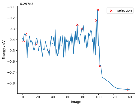
Now it is time to select new data points from our pool. In the following we choose the last-layer gradient kernel as the similarity metric and the max dist selection method (farthest point sampling) to select 10 datapoints from out pool.
[4]:
train_atoms = read(str(cc_train_file_path), ":")
pool_atoms = read("project/benzene.traj", ":")
[5]:
len(pool_atoms)
[5]:
142
[6]:
base_fm_options = {"name": "ll_grad", "layer_name": "dense_2"}
selection_method = "max_dist"

bs = 10

selected_indices = api.kernel_selection(
    "project/models/benzene",
    train_atoms,
    pool_atoms,
    base_fm_options,
    selection_method,
    selection_batch_size=bs,
    processing_batch_size=bs,
)
Computing features: 100%|██████████████████████████████████████| 1142/1142 [00:04<00:00, 273.60it/s]
(1142, 513)
[7]:
selected_indices
[7]:
array([139, 99, 1, 34, 102, 78, 4, 17, 97, 72])
[8]:
energies = np.array([a.get_potential_energy() for a in pool_atoms])
# selected_indices = np.random.randint(0, len(energies), 10)
selection_energies = energies[selected_indices]
As we can see below, the batch selection method only picks a few data points from the optimization part of the pool, indicating that during an optmization the structure of the molecule does not change very much. Hence, there are not many informative samples to be found in it.
[9]:
fig, ax = plt.subplots()

ax.plot(energies)
ax.scatter(selected_indices, selection_energies, marker="x", color="red", label="selection")
ax.set_ylabel("Energy / eV")
ax.set_xlabel("Image")
ax.legend()
[9]:
<matplotlib.legend.Legend at 0x79751d048c50>